Matrix Profile TL;DR
This is a graphic I made to promote the matrix profile. It provides a very quick overview to attract interest.
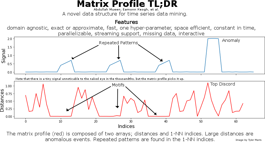
This is a graphic I made to promote the matrix profile. It provides a very quick overview to attract interest.
In part 1 of this series, I introduced a personal conundrum, how can I simplify naming a baby? In this blog post I will discuss how I created clusters of names based on features and sampled them using statistical methods. You do not need a heavy background in statistics or machine learning to follow along.
In order to perform clustering, I needed to identify common traits within names that people consider. When you really start thinking about what you like in a name, it becomes apparent that there is much to consider. Here is a list of features that I derived from names:
Sample name Garen.
1. Percentage of males in the population with this name - 100%
The database of names gives the frequency of individuals with the name since 1880 by both male and female. I simplified it and combined all years into one value. Using the name Garen as an example, you can see that there hasn't been a female with that name on record.
2. Percentage of females in the population with this name - 0%
I used the same logic to compute the percentage of females. Garen was never recorded as a female given name.
3. Percentage of the population with the name
Here I combined the male and female frequency into one value to obtain the popularity of the name.
4. First letter - G
5. First two letters - Ga
6. First three letters - Gar
7. Last letter - n
8. Last two letters - en
9. Last three letters - ren
The beginning and ending letters of a name is pretty easy to obtain by simple string slicing.
10. How to pronounce the name - KRN
I use metaphone to generate this information. It generates a string that creates a sound value. Similar to the name Garen, Karen sounds similar and has the same code of KRN.
11. Number of letters in the name - 5
Here I simply count the number of letters in the name.
Using the same sample name, Garen, here is what all of the features would look like that is fed into the clustering algorithm.
| Feature | Value |
|---|---|
| % Male | 1 |
| % Female | 0 |
| % Population | 0.000232 |
| First letter | g |
| First two letters | ga |
| First three letters | gar |
| Last letter | n |
| Last two letters | en |
| Last three letters | ren |
| Metaphone | krn |
| Length | 5 |
For clustering, I used the NearestNeighbors algorithm from scikit-learn. It provides a supervised and unsupervised approach to clustering. In this case, for baby name recommendation, I set the minimum number of neighbors to 20 and used the automatic algorithm. Once clustering was finished I created a dictionary of similar names.
For example, looking up names similar to Ladon would give us:
['Ladell',
 'Lacy',
 'Little',
 'Lorenza',
 'Lorren',
 'Mikell',
 'Mikal',
 'Laren',
 'Lorin',
 'Laray',
 'Mika',
 'Loren',
 'Larrie',
 'Loran',
 'Lindsey',
 'Lindsay',
 'Micah',
 'Micky',
 'Lester',
 'Mica']
I use the similar names to recommend a name that you may like based on previous likes. The similar names were stored in a Python pickle file and loaded for suggestions while the features of all of the names were stored in a database. The database essentially keeps track of what you like and dislike. This leads us to the more complicated part of the application; sampling.

For sampling, I came up with three strata (groups) with biased weights. These weights are used to compute which group should be sampled from. The weights are multiplied by the number of names that have been liked with a hard cut-off of 10 for the partner and user strata. So if you liked 10 names, the liklihood that it would select a name similar to one that was liked is (liked / total names) user_bias; (10 / 10,832) 0.45. The weights were all calculated this way and normalized from 0 to 1. Once a strata is chosen, I simply selected a name from the cluster group.
To reduce the number of times that you see a name when you dislike it, I added a hard cut-off of two. Essentially, if you did not like a name two or more times, it will never be shown again. This added some necessary logic to check the name that was sampled prior to displaying it. The logic is as follows:
In this post, I illustrated how I created features that were used to cluster names into similar groups. I further illustrated how I used a biased stratified sampling approach to choose a name to show to the user. In the next part of this series I will show you the application and make it freely available.
This post is used to illustrate how to use mass-ts; a library that I created composed of similarity search algorithms in time series data. For this example, I will walk you through similarity search on the UCR data set - robot dog.
The dataset comes from an accelerometer inside a Sony AIBO robot dog. The query comes from a period when the dog was walking on carpet, the test data we will search comes from a time the robot walked on cement (for 5000 data points), then carpet (for 3000 data points), then back onto cement.
Source: https://www.cs.unm.edu/~mueen/Simple_Case_Studies_Using_MASS.pptx
Note
All of the code in this example is using Python 3.
import numpy as np
import mass_ts as mts
from matplotlib import pyplot as plt

%matplotlib inline
robot_dog = np.loadtxt('robot_dog.txt')
carpet_walk = np.loadtxt('carpet_query.txt')
plt.figure(figsize=(25,5))
plt.plot(np.arange(len(robot_dog)), robot_dog)
plt.ylabel('Accelerometer Reading')
plt.title('Robot Dog Sample')
plt.show()

The series data for the robot dog is difficult to see a pattern unless you make the plot very large. At 25 by 5 you can see a pattern in the middle of the data set. This is where the carpet walk takes place.
plt.figure(figsize=(25,5))
plt.plot(np.arange(len(carpet_walk)), carpet_walk)
plt.ylabel('Accelerometer Reading')
plt.title('Carpet Walk Sample')
plt.show()

Now we can search for the carpet walk snippet within the robot dog sample using MASS.
distances = mts.mass3(robot_dog, carpet_walk, 256)
min_idx = np.argmin(distances)
min_idx
The minimum index found is the same as the author claims. We can now visualize this below.
plt.figure(figsize=(25,5))
plt.plot(np.arange(len(robot_dog)), robot_dog)
plt.plot(np.arange(min_idx, min_idx + 100), carpet_walk, c='r')
plt.ylabel('Accelerometer Reading')
plt.title('Robot Dog Sample')
plt.show()

# Plot the carpet walk query
fig, (ax1, ax2, ax3) = plt.subplots(3,1,sharex=True,figsize=(20,10))
ax1.plot(np.arange(len(carpet_walk)), carpet_walk)
ax1.set_ylabel('Carpet Walk Query', size=12)

# Plot use case best match from original authors
ax2.plot(np.arange(100), robot_dog[7478:7478+100])
ax2.set_ylabel('Original Best Match', size=12)

# Plot our best match
ax3.plot(np.arange(100), robot_dog[min_idx:min_idx+100])
ax3.set_ylabel('Our Best Match', size=12)

plt.show()
