Introduction

In this quick post covering descriptive statistics we will cover the mode. The mode describes the frequency of values within a given data set. To learn about the median or mean, please click the respective links.

Mode

The mode is one of the easiest descriptive statistics to understand. It simply provides the value(s) that occur(s) most frequently. In most cases it is not very informative to identify a single value that occurs frequently, however it is useful to find the number of occurences for many values. To do this we can make use of a histogram to display the data.

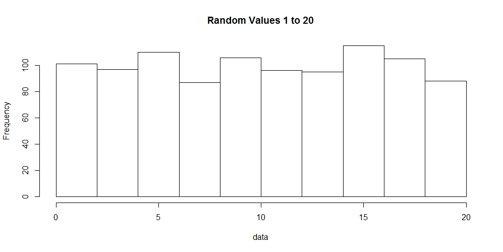
Lets generate 1,000 numbers in the range of 1 to 20 and visualize it. The code to do this in R follows:

data <- sample(1:20, 1000, replace=T)
hist(data, main="Random Values 1 to 20")

In the code sample above we generated the numbers and created a histogram of the data. A histogram, shown below, displays the number of occurrences for each value observed in our data set.

R

Unfortunately, there is not a single function to obtain the mode of a given data set. However, we can create a table for the number of occurrences or visualize the data with a histogram.

data <- c(1, 1, 2, 3, 3, 3, 4, 5, 5, 5, 5, 5)
table(data)

Python

In the Scipy module we can obtain the mode only.

from scipy import stats
data = [1, 1, 2, 3, 3, 3, 4, 5, 5, 5, 5, 5]
stats.mode(data)

We can also use Scipy to reproduce a frequency table.

from scipy import stats
data = [1, 1, 2, 3, 3, 3, 4, 5, 5, 5, 5, 5]
stats.itemfreq(data)

Conclusion

The mode is one of the most under used descriptive values of a data set. It simply provides you with what value occurs most frequently. In some instances it might be nice to know, but less useful than the median or mean. R does not provide a built in method for finding the mode by itself, however Python's Scipy module provides both frequencys of all values or simply the mode.

In the next post we will look at some real world applications of the mean, median and mode.

Introduction

In this next post on descriptive statistics, the median will be discussed. In part 1 of this blog series we learned about the mean (average) and found out that it can easily be skewed by large or small values. Both the median and mean are "measures of central tendency". Central tendency is essentially the center position of a distribution for a data set. Now that you are refreshed, we can discuss the median.

Median

The median is simple to calculate. First, we must arrange the values from least to greatest. Next, we pick the center value - this is our median when there is an odd number of values. When there are an even number of values we simply add the two center values together and divide by 2.

Here are examples of both odd and even cases:

Odd number of values

1, 2, 3, 4, 5
Median = 3

Even number of values

1, 2, 3, 4
Median = (2 + 3) / 2 = 2.5

Median vs. Mean

As you can see the median is not influenced by outliers. It provides the central value that most of us tend to think of as the average (mean). You might ask when you would use one over the other. This question is difficult to answer without context. In some situations it may make more sense to use one or both. Let's look at some grades for 10 random students to see how the mean and median look.

The raw values are as follows:

20, 20, 25, 27, 29, 37, 45, 55, 90, 100

In the plot, shown above, the blue line represents the mean - 44.8%. The green line represents the median - 33%. Clearly there is a difference between these two measures of central point.

R

To calculate the median in R - simply use the built in function.

grades <- c(20, 20, 25, 27, 29, 37, 45, 55, 90, 100)
median_grade <- median(grades)

Python

To calculate the median in Python we use Numpy. Import Numpy and use the median function.

import numpy as np
grades = [20, 20, 25, 27, 29, 37, 45, 55, 90, 100]
median_grade = np.median(grades)

Conclusion

In this post we discussed the median and how it differentiates from the mean. We also established that context is important when deciding to use one versus the other. The mean and median are important values used in statistics and our every day lives.

The next article will discuss the mode - another useful descriptive statistic.

Introduction

Descriptive statistics is a meaningful part of statistics in which a value provides informative insight about a particular data set. Some examples of descriptive stastics include the values mean, median and mode. In this post I will provide some concepts of the mean and how to calculate this value using both R and Python. All of the examples in Python will make use of the library SciPy or Numpy.

Mean

The mean provides an average of the observed values. It can be useful to show a simple summary illustrating the average, however it can become very misleading. Keep in mind that the terms mean and average can be used interchangeably.

Let's look at the following numbers:

Set 1
1, 2, 3, 4, 5, 6, 7

Set 2
1, 2, 3, 4, 5, 20, 100

In set 1 the average is meaningful as it respresents a fair distribution of the values. However, in set 2 the average is right skewed due to the large numbers. In other words, the mean does not represent the majority of the observations. Imagine if these sets represented exam scores. This would mean that average for set 1 is 4% and average of set 2 is 21.67%. You should get the idea that only 2 students in set 2 performed well while the majority of the students performed very poorly. It is very important to know the underlying data and how the mean represents it.

The two plots above provide a better illustration of how skewed the data becomes with larger values. The red line marks the average. Keep in mind that this can happen with very small values as well.

R

In R it is very easy to calculate the mean. Below, we create a variable to hold some values and simply use the built-in mean function.

my_data = c(1,2,3,4,5)
mean(my_data)

Python

Similarly Python makes it very easy to calculate the mean. Ensure that you have the Numpy package installed to follow this snippet.

import numpy as np

my_data = [1,2,3,4,5]
np.mean(my_data)

Conclusion

The mean is a very useful but sometimes misleading descriptive statistic. It is very common to hear about averages in our daily lives, but you should know that it may not always be a good representation of the data.

The next article will cover the median - another useful descriptive statistic that is not as fragile.